color를 사용하는 방법은 모두 같다. 그냥 color인자에 값을 주면 된다. 다만 표현 방식에 차이가 있을 뿐이다.
1. Named colors
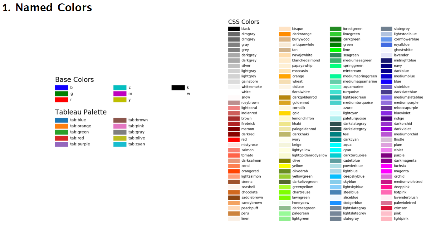
ax.text(color=c)

# Base color의 b, c, g는 외우고 있지 않으면 뭔지 모를 수도 있기 때문에 좀 더 명시적인 방법으로 Tableau palette를 사용합니다.
ax.text(color='tab:blue')

ax.text(color= 'darkblue')
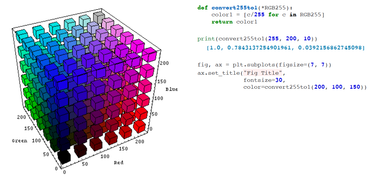
2. RGB colors
좀 더 디테일하게 색깔을 정하기 위해 RGB컬러를 사용할 수도 있다. 다만 Matplotlib에서는 스케일을 0~1사이로 조정해줘야 하는 것 같다.
3. Colormaps
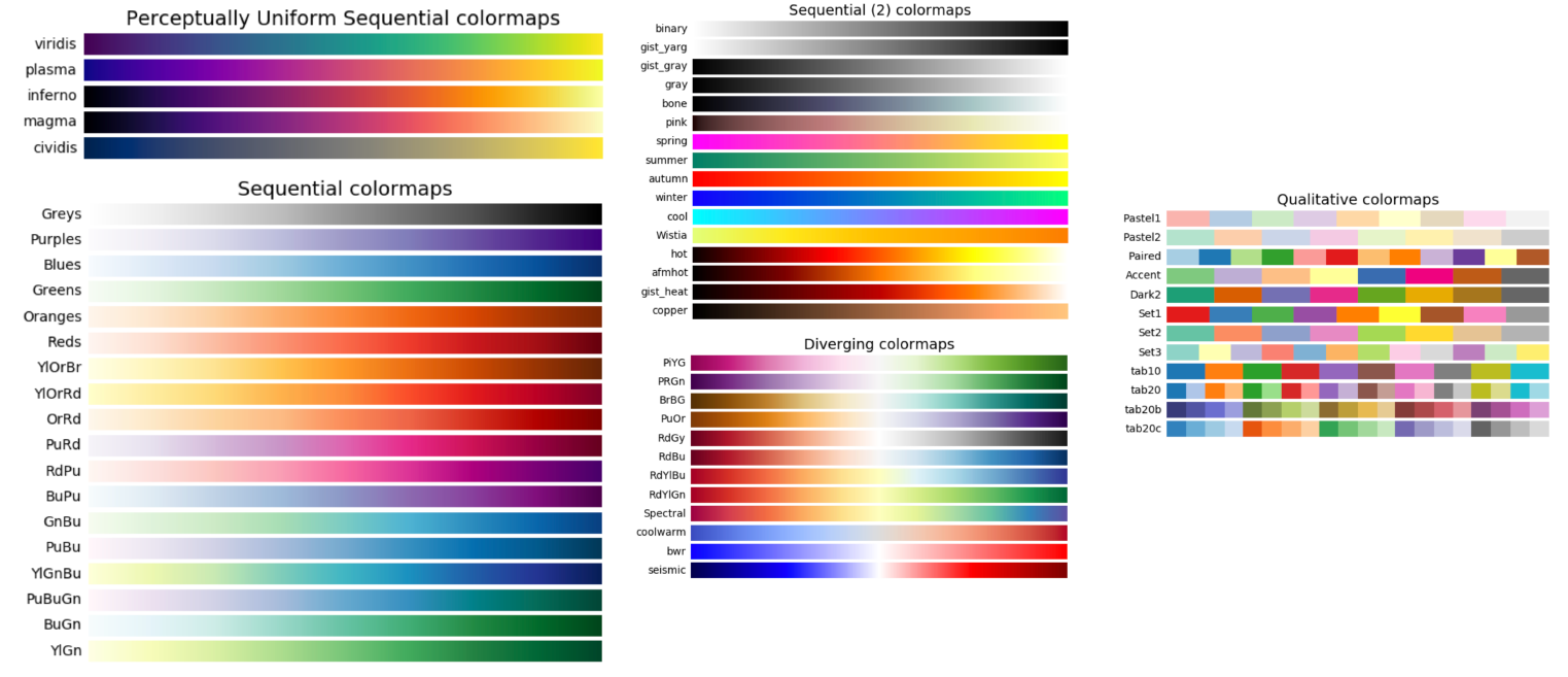
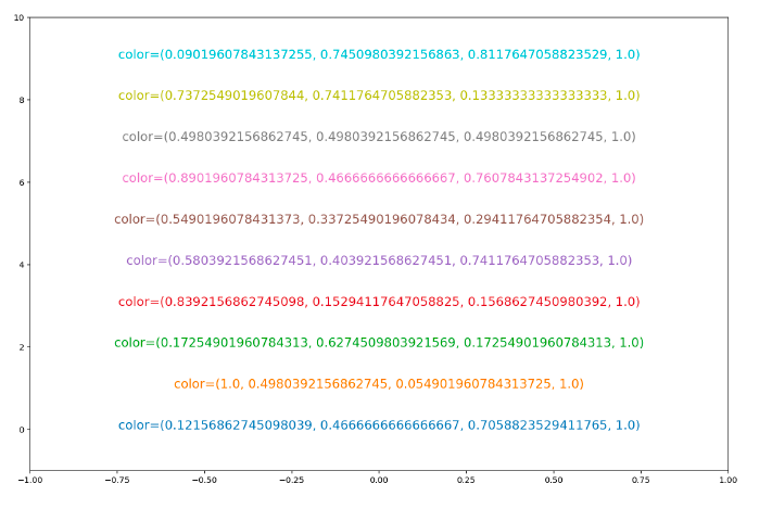
1) discrete한 colormap
import matplotlib.cm as cm

cmap = cm.get_cmap('tab10')

print(cmap.colors)
-----------------------------------------------------------
((0.12156862745098039, 0.4666666666666667, 0.7058823529411765), (1.0, 0.4980392156862745, 0.054901960784313725), (0.17254901960784313, 0.6274509803921569, 0.17254901960784313),
(0.8392156862745098, 0.15294117647058825, 0.1568627450980392), (0.5803921568627451, 0.403921568627451, 0.7411764705882353), (0.5490196078431373, 0.33725490196078434, 0.29411764705882354),
(0.8901960784313725, 0.4666666666666667, 0.7607843137254902), (0.4980392156862745, 0.4980392156862745, 0.4980392156862745), (0.7372549019607844, 0.7411764705882353, 0.13333333333333333),
(0.09019607843137255, 0.7450980392156863, 0.8117647058823529))

cmap(0)
--------------------------------------
(0.12156862745098039, 0.4666666666666667, 0.7058823529411765, 1.0)
fig, ax = plt.subplots(figsize=(15, 10))
ax.set_ylim([-1, len(cmap.colors)])
for i in range(len(cmap.colors)):
    ax.text(0, i, "color="+str(cmap(i)), color=cmap(i))
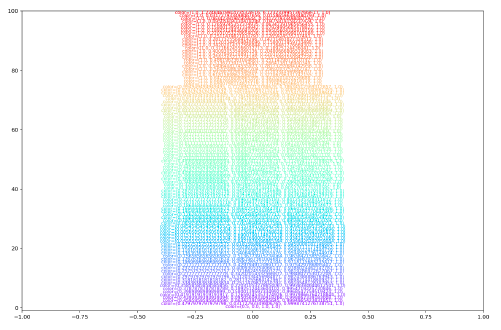
2) continuous한 colormap
import matplotlib.cm as cm

cmap = cm.get_cmap('rainbow', lut=100)

fig, ax = plt.subplots(figsize=(15, 10))
ax.set_ylim([-1, 100])
for i in range(100):
    ax.text(0, i, "color="+str(cmap(i)), color=cmap(i))
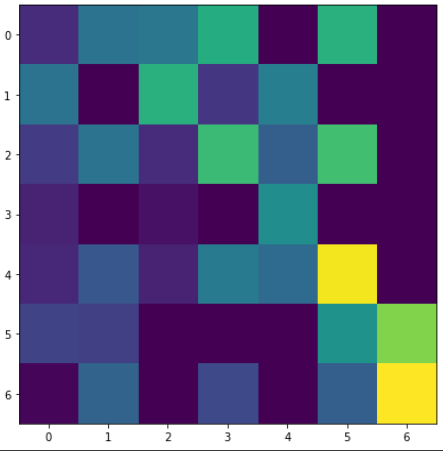
3) Auto colormap
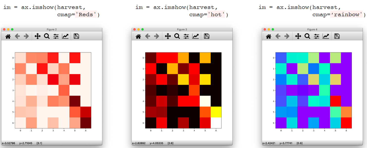
# ax.imshow()
harvest = np.array([[0.8, 2.4, 2.5, 3.9, 0.0, 4.0, 0.0],
[2.4, 0.0, 4.0, 1.0, 2.7, 0.0, 0.0],
[1.1, 2.4, 0.8, 4.3, 1.9, 4.4, 0.0],
[0.6, 0.0, 0.3, 0.0, 3.1, 0.0, 0.0],
[0.7, 1.7, 0.6, 2.6, 2.2, 6.2, 0.0],
[1.3, 1.2, 0.0, 0.0, 0.0, 3.2, 5.1],
[0.1, 2.0, 0.0, 1.4, 0.0, 1.9, 6.3]])

fig, ax = plt.subplots(figsize=(7, 7))
ax.imshow(harvest)
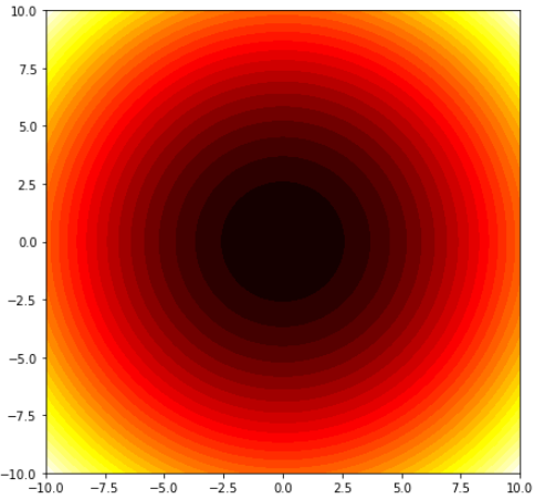
# ax.contourf()
x = np.linspace(-10, 10, 100)
y = x
X, Y = np.meshgrid(x, y)
Z = np.power(X, 2) + np.power(Y, 2)
levels = np.linspace(np.min(Z), np.max(Z), 30)
fig, ax = plt.subplots(figsize=(7, 7))

ax.contourf(X, Y, Z, levels=levels, cmap='hot')
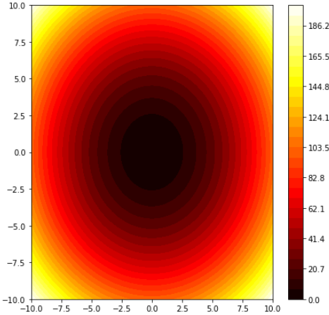
x = np.linspace(-10, 10, 100)
y = x
X, Y = np.meshgrid(x, y)
Z = np.power(X, 2) + np.power(Y, 2)
levels = np.linspace(np.min(Z), np.max(Z), 30)
fig, ax = plt.subplots(figsize=(7, 7))
cf = ax.contourf(X, Y, Z,
levels=levels,
cmap='hot')

cbar = fig.colorbar(cf)
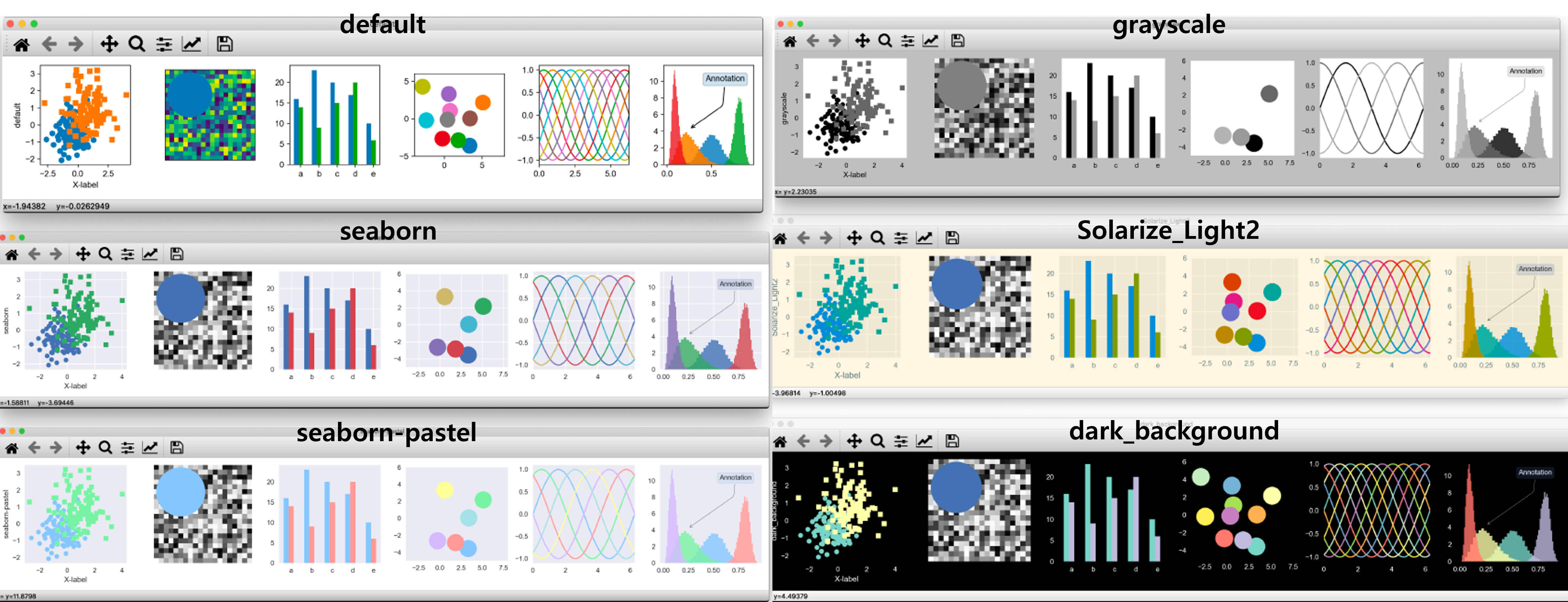
4. Style
plt.style.available
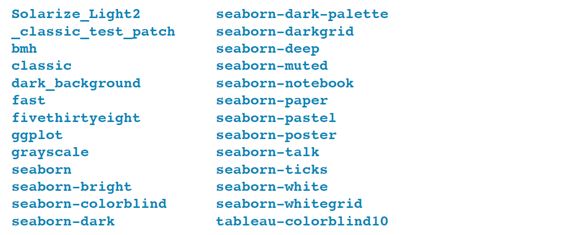
plt.style.use('seaborn')