
판다스 데이터 분석하기
이번 포스트에서는 DataFrame으로부터 의미 있는 정보(insight)를 얻기 위해 데이터를 분석하는 방법에 대해 알아보겠습니다. 이 전 포스트까지는 직접 만든 작은 데이터셋에 대해 했지만, 이번 포스트에서는 외부에서 가져온 데이터셋을 이용해 분석에 사용해 보도록 하겠습니다.
데이터 셋: FIFA19 complete player dataset
1. 통계적 분석(Statistical Data Analysis)
# 필요한 라이브러리 불러오기
import pandas as pd
# 데이터 읽어서 가져오기
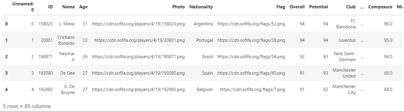
df = pd.read_csv("../input/fifa19/data.csv")
df.head(5)
# df.tail()
df.shape
-------------------
(18207, 89)
df.columns
--------------------------------------------------------------------------------
Index(['Unnamed: 0', 'ID', 'Name', 'Age', 'Photo', 'Nationality', 'Flag',
       'Overall', 'Potential', 'Club', 'Club Logo', 'Value', 'Wage', 'Special',
       'Preferred Foot', 'International Reputation', 'Weak Foot',
       'Skill Moves', 'Work Rate', 'Body Type', 'Real Face', 'Position',
       'Jersey Number', 'Joined', ...
        'GKPositioning', 'GKReflexes', 'Release Clause'],
      dtype='object')
df.info()
----------------------------------------------------------------------------
<class 'pandas.core.frame.DataFrame'>
RangeIndex: 18207 entries, 0 to 18206
Data columns (total 89 columns):
 #   Column                    Non-Null Count  Dtype
---  ------                    --------------  -----
 0   Unnamed: 0                18207 non-null  int64
 1   ID                        18207 non-null  int64
 2   Name                      18207 non-null  object
 3   Age                       18207 non-null  int64
 4   Photo                     18207 non-null  object
 5   Nationality               18207 non-null  object
 6   Flag                      18207 non-null  object
 7   Overall                   18207 non-null  int64
 8   Potential                 18207 non-null  int64
 9   Club                      17966 non-null  object
 ...
 86  GKPositioning             18159 non-null  float64
 87  GKReflexes                18159 non-null  float64
 88  Release Clause            16643 non-null  object
dtypes: float64(38), int64(6), object(45)
memory usage: 12.4+ MB
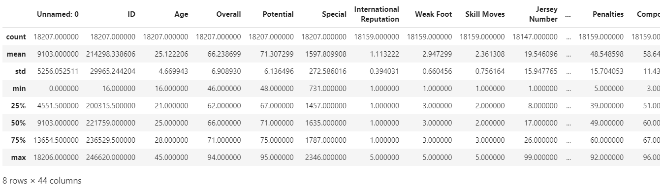
df.describe()
df['Position'].unique()
------------------------------------------------------
array(['RF', 'ST', 'LW', 'GK', 'RCM', 'LF', 'RS', 'RCB', 'LCM', 'CB',
       'LDM', 'CAM', 'CDM', 'LS', 'LCB', 'RM', 'LAM', 'LM', 'LB', 'RDM',
       'RW', 'CM', 'RB', 'RAM', 'CF', 'RWB', 'LWB', nan], dtype=object)
# aggregation 함수

df['Overall'].mean()
----------------------------------
66.23869940132916

df['Age'].max()
--------------------
45

# aggregation 함수를 DataFrame에 대해 적용하면 각 column별로 aggregation함수가 적용된다
df.max()
-------------------------------------------
Unnamed: 0                                                         18206
ID                                                                246620
Name                                                       Óscar Whalley
Age                                                                   45
Photo                       https://cdn.sofifa.org/players/4/19/9833.png
Nationality                                                     Zimbabwe
Flag                                 https://cdn.sofifa.org/flags/99.png
Overall                                                               94
Potential                                                             95
Club Logo                   https://cdn.sofifa.org/teams/2/light/983.png
Value                                                                €9M
Wage                                                                 €9K
Special                                                             2346
International Reputation                                             5.0
Weak Foot                                                            5.0
Skill Moves                                                          5.0
Jersey Number                                                       99.0
Crossing                                                            93.0
2. 탐색적 분석(Exploratory Data Analysis)
1) Selection과 Filtering
# selection
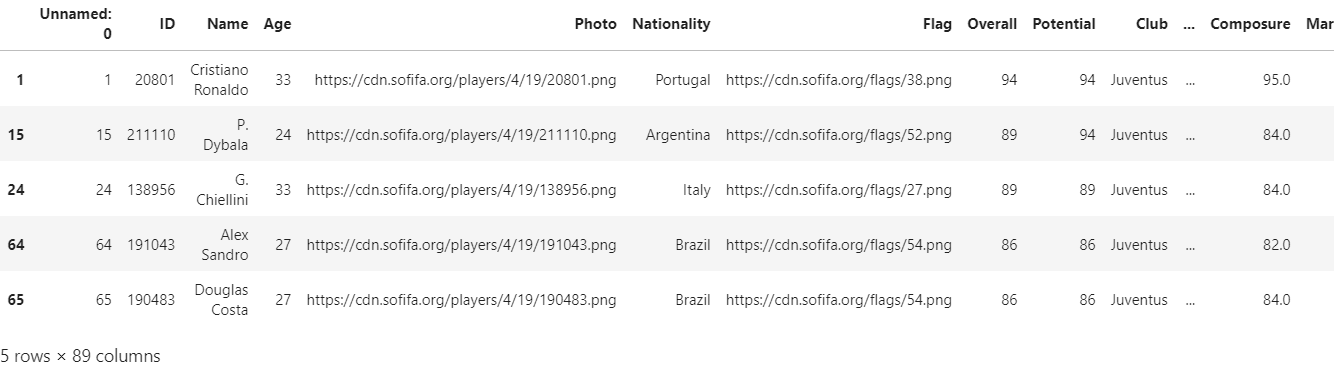
condition = df['Club'] == 'Juventus'
df[condition].head(5)
# filtering
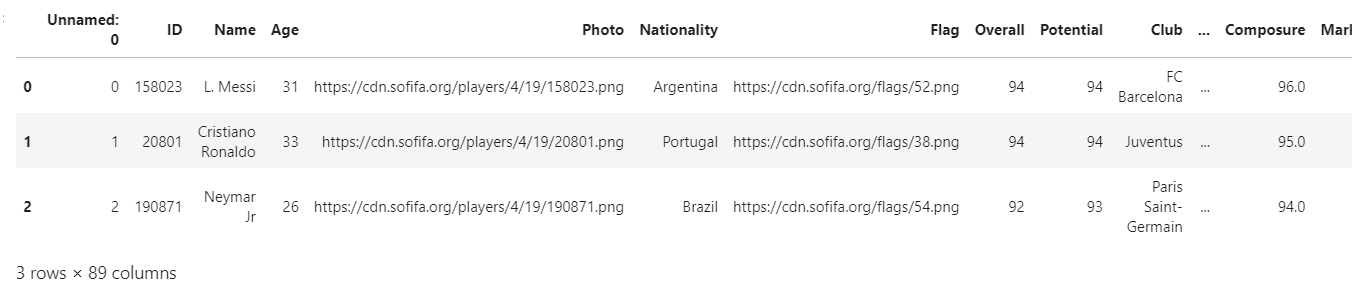
condition = df['Overall'] > 91
df[condition]
# selection & filtering
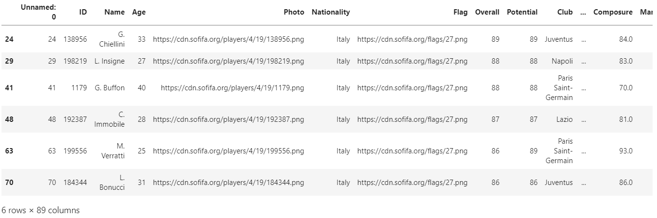
condition_1 = df['Nationality'] == 'Italy'
condition_2 = df['Overall'] >= 85
df[condition_1 & condition_2]
# selection & aggregation

condition = df['Position'] == 'GK'


df[condition][['GKDiving', 'GKHandling', 'GKPositioning', 'GKReflexes']].mean()
----------------------------------------------------------------------------------------
GKDiving         65.323951
GKHandling       62.868148
GKPositioning    63.047407
GKReflexes       66.101728
dtype: float64


df[condition][['GKDiving', 'GKHandling', 'GKPositioning', 'GKReflexes']].mean(axis=1)
----------------------------------------------------------------------------------------
3        89.25
9        88.75
18       86.75
19       87.50
22       87.50
         ...
18178    47.25
18180    47.25
18183    47.00
18194    47.00
18198    47.00
Length: 2025, dtype: float64
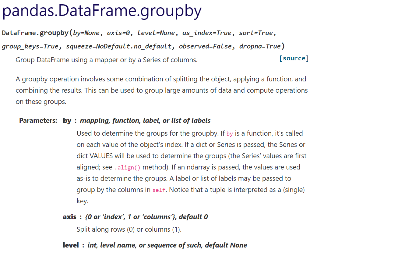
2) Groupby
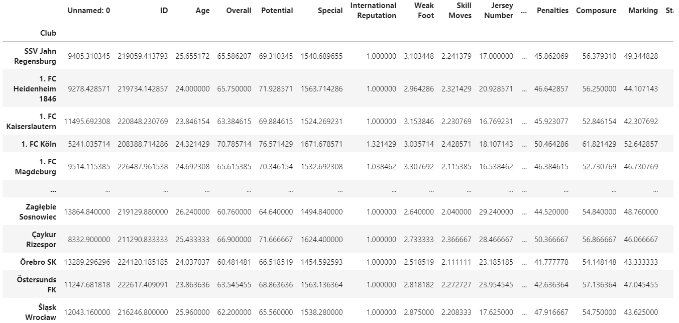
df.groupby(by='Club').mean()
df[['Club', 'Nationality', 'Name']].groupby(by=['Club', 'Nationality']).count()

df.groupby(by=['Club', 'Nationality'])[['Age', 'Overall', 'Potential']].mean()

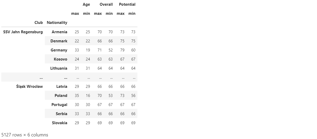
df.groupby(by=['Club', 'Nationality'])[['Age', 'Overall', 'Potential']].agg([max, min])
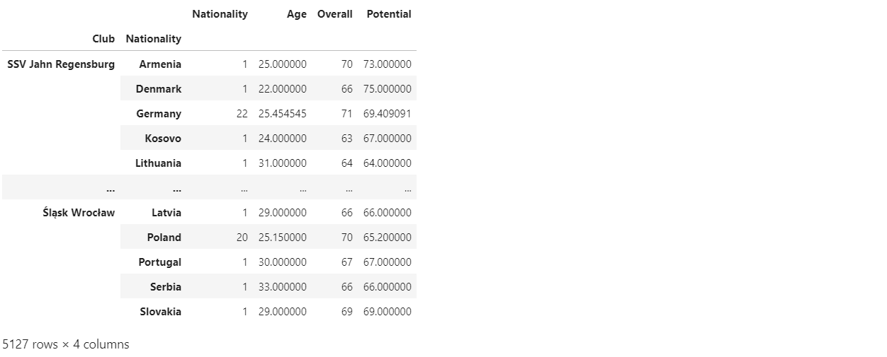
df.groupby(by=['Club', 'Nationality']).agg({'Nationality': 'count', 'Age': 'mean', 'Overall': 'max', 'Potential': 'mean'})
3. 분석에 유용한 함수들
# DataFrame.sort_values(by = 'col', ascending=False, replace=True)
# Series.value_counts()
# DataFrame.apply()
# Series.apply()
# Groupby.apply()